1
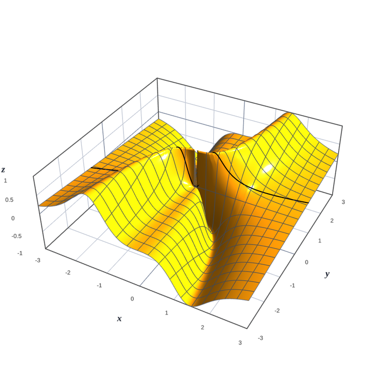
unit_7_g_7_1
Manipulate[
2
unit_23_gd
Manipulate[Module[{gridPoints$ = Range[-5, 5, 1], arrowScale
3
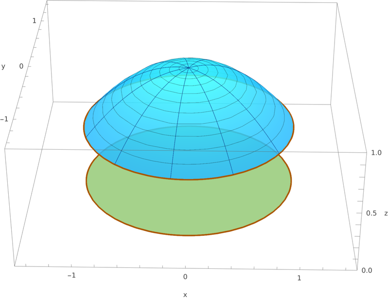
unit_17_gd
Manipulate[
4
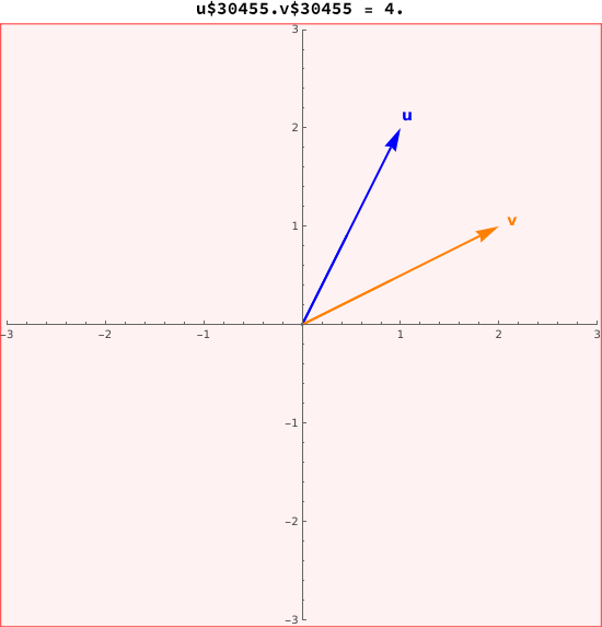
unit_1_g_1_2
Manipulate[Module[{u = {1, 2}, v, angle, dp}, v = RotationTr
5

unit_11_gd
DynamicModule[{zoom = 1.0},
6
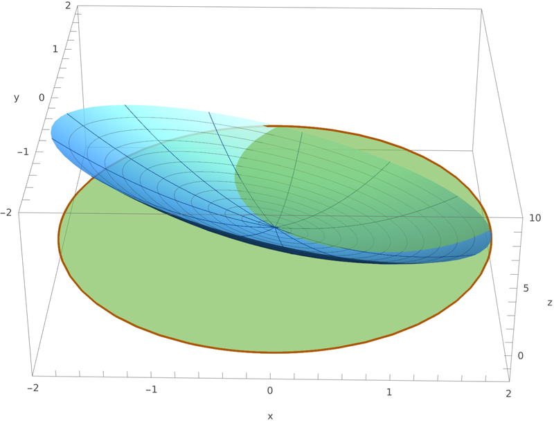
unit_13_gd
Manipulate[Show[Plot3D[0, {x, -2, 2}, {y, -2, 2}, PlotStyle
7
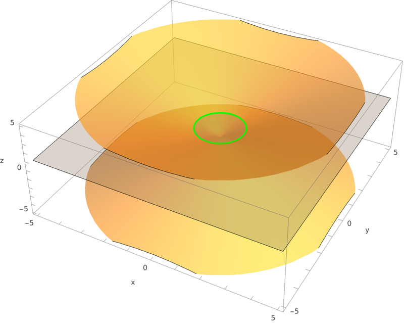
week_3_ie_1
Manipulate[Module[{surfpos$, surfneg$, planeZ$, curveZ$, pla
8
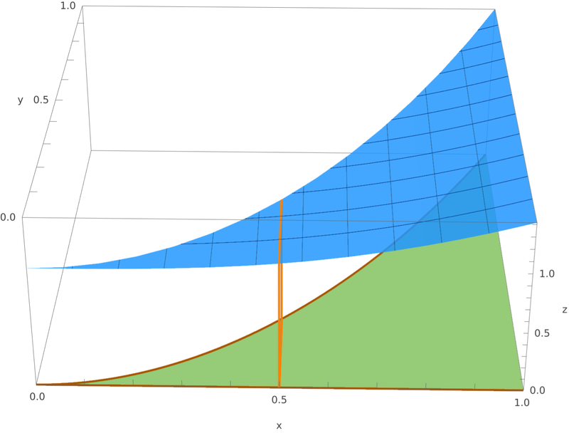
unit_15_gd
Manipulate[Show[Plot3D[0, {x, 0, 1}, {y, 0, 1}, PlotStyle ->
9
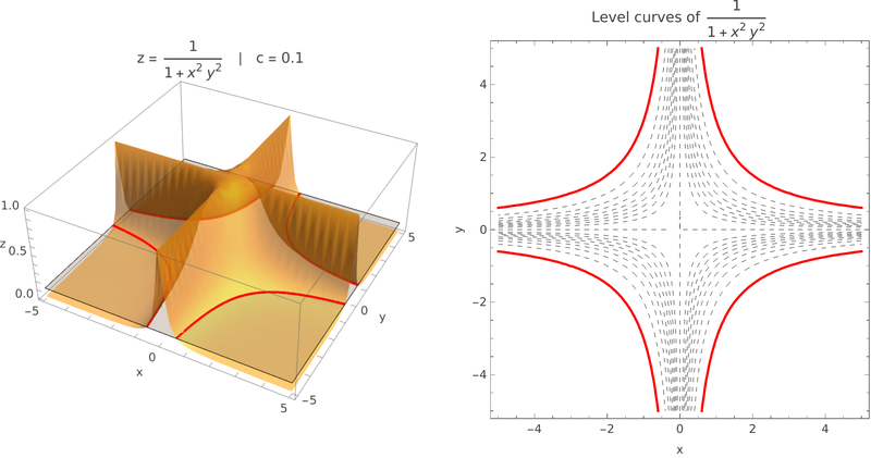
unit_6_g_6_1
Manipulate[Module[{surf, plane, intersect, contourplot, high
10
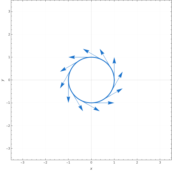
unit_22_gd
Manipulate[Module[{a = 2*t + (1 - t)*1, b = 2*s + (1 - s)*1,
11
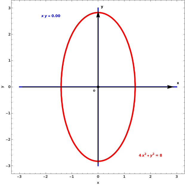
unit_12_gd
Manipulate[
12
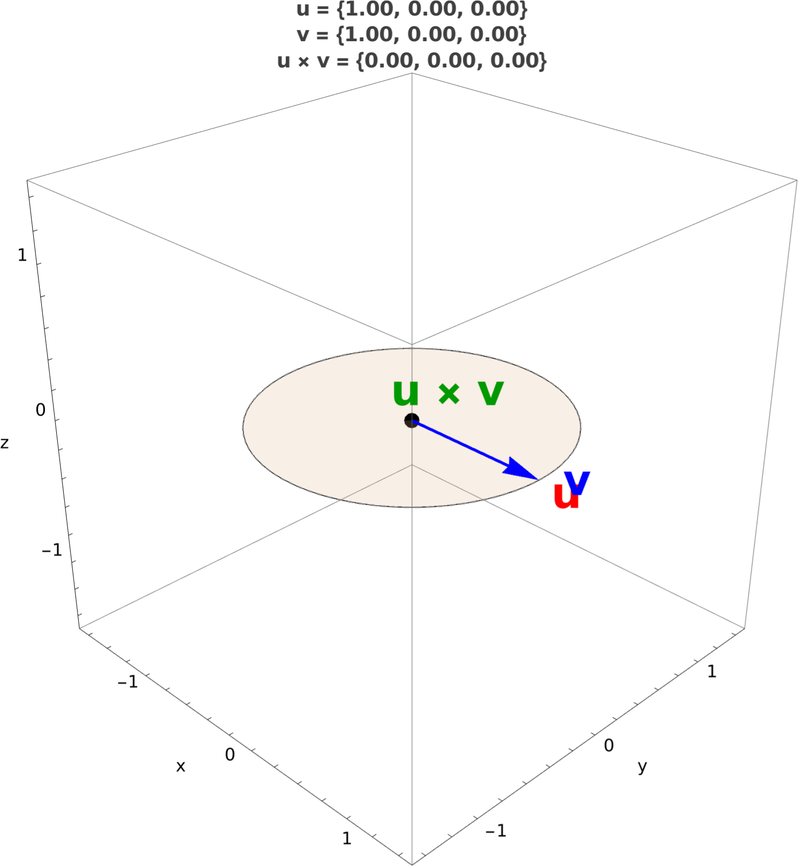
unit_2_g_2_3
Manipulate[Module[{u, v, crossProduct}, u = {1, 0, 0}; v = {
13
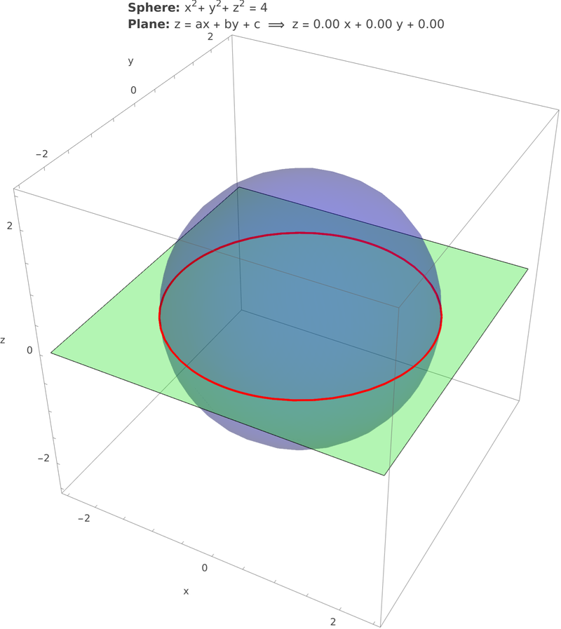
unit_1_ie_2
Manipulate[Module[{n$, nNorm$, radius2$, d$, u$, v$, center$
14
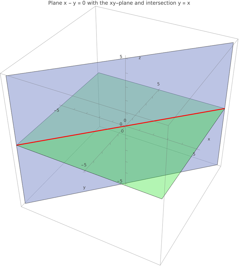
unit_1_ie_3
Manipulate[Show[{If[showPlane, ContourPlot3D[x - y == 0, {x,
15
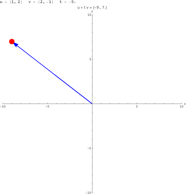
unit_1_ie_1
Manipulate[Column[{Row[{"u = ", {1, 2}, Spacer[20], "v = ",
16
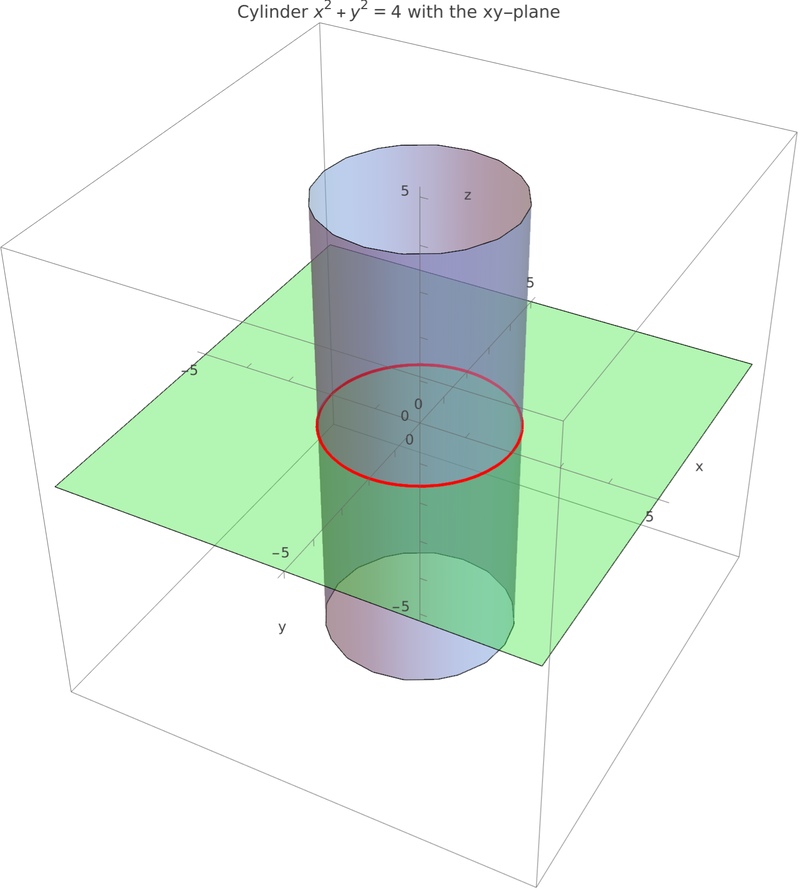
unit_1_ie_4
Manipulate[Show[{If[showSurface, ContourPlot3D[x^2 + y^2 - 4
17
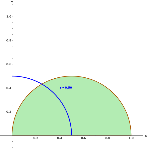
unit_16_gd
Manipulate[Show[Plot[0, {x, -0.1, 1.1}, PlotStyle -> Opacity
18
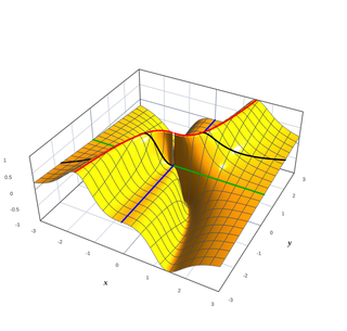
unit_7_g_7_1
Manipulate[
19
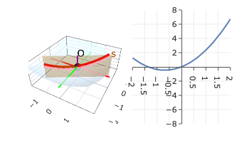
unit_9_g_9_1
Manipulate[
20
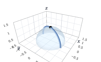
unit_8_g_8_1
Manipulate[
21
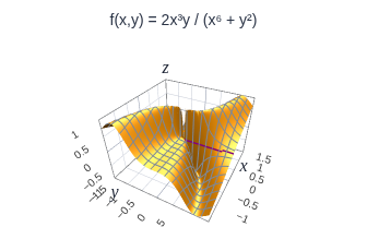
demo_discontinuity_q
Manipulate[
22
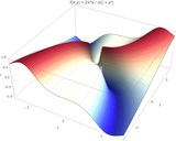
demo_discontinuity
Manipulate[
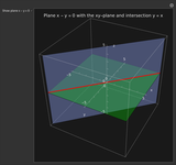
23
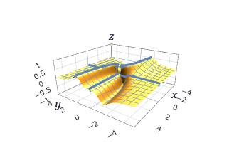
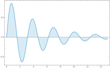
Manipulate[
24
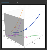
demo_chainrule
Manipulate[
25
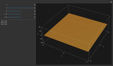
unit_3_g_3_1
Manipulate[Module[{surf, planeZ, curveZ, planeX, curveX, pla
26
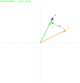
unit_2_g_2_2
Manipulate[Module[{u = {1, 2}, v0 = {2, 1}, v, proj, orth, p
27
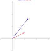
demo_quadric_curves
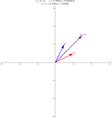
Manipulate[
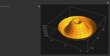
28
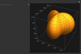
demo_vertex_ecc3
Manipulate[
29
demo_vertex_ecc
Manipulate[
30
demo_quadric_family
Manipulate[
31
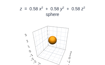
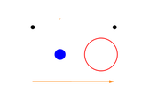
demo_quadric_sphere
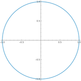
Manipulate[
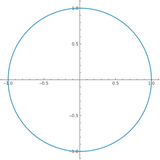
32
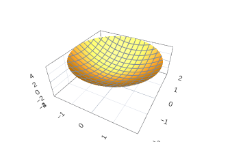
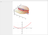
pr
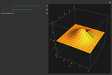
Manipulate[Plot3D[x^2 - c y^2, {x, -2, 2}, {y, -2, 2}, PlotR
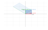
33
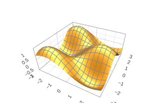
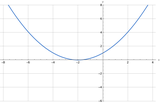
sincos
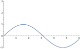
Manipulate[Plot3D[Sin[a x] Cos[b y],{x,-3,3},{y,-3,3}],{a,0.
34
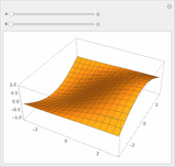
Manipulate[Plot3D[Sin[a x] Cos[b y],{x,-3,3},{y,
35
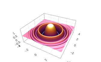
ripples
Manipulate[Plot3D[Cos[k (x^2 + y^2)] Exp[-(x^2 + y^2)/6], {x
36
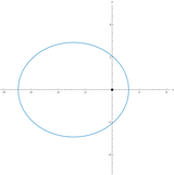
demo_conic_family
Manipulate[
37
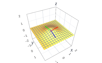
tangents1
Manipulate[
38
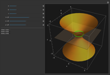
week_3_ie_2
Manipulate[Module[{surfpos$, surfneg$, planeZ$, curveZ$, pla
39
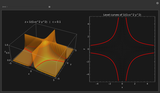
unit_6_g_6_1
Manipulate[Module[{surf, plane, intersect, contourplot, high
40
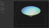
unit_19_gd
Manipulate[Show[Plot3D[0, {x, -2, 2}, {y, -2, 2}, PlotStyle
41
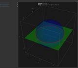
unit_1_ie_4
Manipulate[Module[{n$, nNorm$, radius2$, d$, u$, v$, center$
42
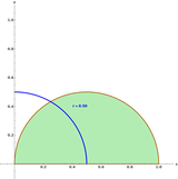
unit_16_gd
Manipulate[Show[Plot[0, {x, -0.1, 1.1}, PlotStyle -> Opacity
43
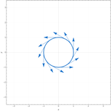
unit_21_gd
Manipulate[Module[{a$ = 2*t + (1 - t)*1, b$ = 2*s + (1 - s)*
44
unit_1_ie_3
Manipulate[Column[{Row[{"u = ", {1, 2}, Spacer[20], "v = ",
45
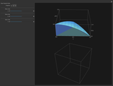
unit_18_gd
Manipulate[Column[{Row[{Show[Plot3D[0, {x, 0, 1}, {y, 0, 1},
46
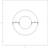
unit_25_gd
Manipulate[Show[Graphics[{{GrayLevel[0.9], Thin, Table[Line[
47
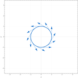
week_22
Manipulate[Module[{a = 2*t + (1 - t)*1, b = 2*s + (1 - s)*1,
48
unit_23_gd
Manipulate[Module[{gridPoints$ = Range[-5, 5, 1], arrowScale
49
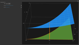
unit_15_gd
Manipulate[Show[Plot3D[0, {x, 0, 1}, {y, 0, 1}, PlotStyle ->
50
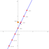
week_2_ie_2
Manipulate[Module[{lineFunc$, points$, midIndex$, P$, select
51
unit_24_gd_2
Manipulate[Module[{radius$ = (6/8)*Min[1 - x0, 1 + x0, 1 - y
52
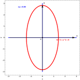
week_12
Manipulate[
53
unit_24_gd_1
Manipulate[Module[{gridPoints$ = Range[-5, 5, 1], arrowScale
54
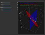
week_2_ie_1
Manipulate[Module[{p1$ = {1, 2, 3}, n1$ = {1, 0, 0}, p2$ = {
55
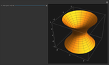
demo_u3_quadric
Manipulate[
56
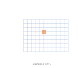
demo_u20_jacobian
Manipulate[Module[{m, jac},
57
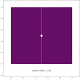
demo_u17_com
Manipulate[Module[{xbar},
58
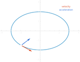
demo_u5_bead
Manipulate[Dynamic[Module[{tt, p, vv, aa},
59
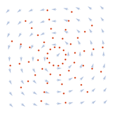
demo_u21_flow
Manipulate[Dynamic[Module[{tau},
60
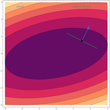
demo_u10_gradlevel
Manipulate[Module[{f, gx, gy, n},
61
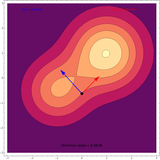
demo_u9_dirderiv
Manipulate[Module[{f, fx, fy, gx, gy, du},
62
time_split
Manipulate[Dynamic[If[!ListQ[buf2],buf2={}];AppendTo[buf2,Cu
63
live_clock
Manipulate[Dynamic[Graphics[{Circle[{0,0},1],Table[Line[{0.9
64
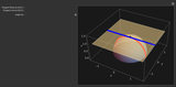
unit_8_gd
Manipulate[Show[ParametricPlot3D[{Cos[phi]*Sin[psi], Sin[phi
65
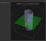
unit_1_ie_2
Manipulate[Show[{If[showSurface, ContourPlot3D[x^2 + y^2 - 4
66
unit_1_ie_1
Manipulate[Show[{If[showPlane, ContourPlot3D[x - y == 0, {x,
67
live-damped-frame
Manipulate[Plot[Sin[a x] Exp[-x/5], {x, 0, 15}, Frame -> Tru
68
live-gaussian-blue
Manipulate[Plot3D[Exp[-(x^2 + y^2)/a], {x, -2, 2}, {y, -2, 2
69
live-rainbow-surface
Manipulate[Plot3D[Sin[a x y], {x, 0, 3}, {y, 0, 3}, Mesh ->
70
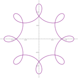
live-parametric-styled
Manipulate[ParametricPlot[{Cos[t] + a Cos[7 t]/2, Sin[t] - a
71
live-helix-points
Manipulate[ListPointPlot3D[Table[{Cos[t], Sin[t], a t/10}, {
72
live-listplot3d
Manipulate[ListPlot3D[Table[Sin[a i] Cos[j], {i, 0, 3, 0.25}
73
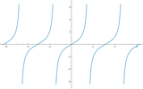
live-tan
Manipulate[Plot[Tan[a x], {x, -2 Pi, 2 Pi}], {{a, 1}, 0.5, 2
74
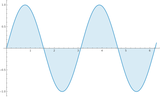
live-filling
Manipulate[Plot[Sin[a x], {x, 0, 2 Pi}, Filling -> Axis], {{
75
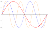
live-plot-styles
Manipulate[Plot[{Sin[x], Sin[2 x], Sin[a x]}, {x, 0, 2 Pi},
76
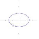
unit_5_g_5_1
Manipulate[With[{curve = ParametricPlot[{3*Cos[t], 2*Sin[t]}
77
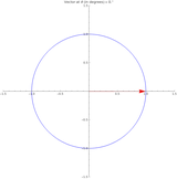
unit_4_g_4_1
Manipulate[Graphics[{Blue, Circle[{0, 0}, 1], Red, Arrow[{{0
78
unit_2_g_2_1
Manipulate[Module[{u = {1.3, 1.7}, v = {1, 0.5}, proj, orth}
79
unit_1_g_1_1
Manipulate[Module[{u = {1, 2}, v0 = {2, 1}, v, w}, v = len*N
80
live-revolution
Manipulate[RevolutionPlot3D[Sin[a x] + 2, {x, 0, 2 Pi}], {{a
81
live-spherical
Manipulate[SphericalPlot3D[1 + a Sin[3 p] Sin[t], {t, 0, Pi}
82
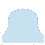
live-region
Manipulate[RegionPlot[x^2 + y^3 < a, {x, -2, 2}, {y, -2, 2}]
83
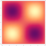
live-density
Manipulate[DensityPlot[Sin[a x] Sin[y], {x, -3, 3}, {y, -3,
84
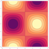
live-contour
Manipulate[ContourPlot[Sin[a x] Cos[y], {x, -3, 3}, {y, -3,
85
Manipulate[ImageRotate[Blur[CurrentImage[],b],th
86
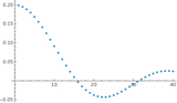
live-listplot
Manipulate[ListPlot[Table[{i,Sin[a i]/i},{i,1,40}],ImageSize
87
live-spheres
Manipulate[Graphics3D[{Orange,Sphere[{0,0,0},r],Blue,Sphere[
88
live-torus-knot
Manipulate[ParametricPlot3D[{Cos[t](2+Cos[a t]),Sin[t](2+Cos
89
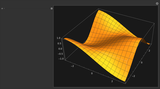
live-surface
Manipulate[Plot3D[Sin[a x] Cos[y],{x,-3,3},{y,-3,3},ImageSiz
90
live-graphics-primitives
Manipulate[Graphics[{Blue,Disk[{0,0},r],Red,Thick,Circle[{1.
91
live-polar-rose
Manipulate[PolarPlot[1+a Cos[5 t],{t,0,2 Pi},ImageSize->380]
92
rose
Manipulate[ParametricPlot[{Cos[t]+a Cos[3 t],Sin[t]-a Sin[3
93
Manipulate[
94
tangents
Manipulate[
95
Manipulate[
96
Manipulate[Plot[a (x/2 + 1)^2, {x, -8, 4}, PlotR
97
Manipulate[Plot[Sin[a x]+b,{x,0,6},PlotRange->{{
98

polymod
Manipulate[Graphics[{PointSize[0.0022], Point[Table[{x, Mod[
99
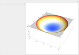
Manipulate[Plot3D[x^2 - c y^2, {x, -2, 2}, {y, -
100
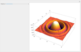
Manipulate[Plot3D[Cos[k (x^2 + y^2)] Exp[-(x^2 +
101

fractal
Image[Table[Length@NestWhileList[(# - UnitStep@Re[# - 1.2])^